Beyond Compactness: A New Measure to Evaluate Congressional Districts

Redrawing congressional district boundaries, an activity that happens every ten years following the decennial census, may be the most consequential application of geography in the United States. As congressional elections have become less competitive, many are raising questions about the current boundaries of congressional districts, often citing lack of geographical compactness as their rationale. Geographical compactness generally ranges from 0 to 1, with 1 being a perfect circle. Wyoming’s only district is currently the most geographically compact district with a score of .77.

The U.S. Supreme Court has ruled multiple times that the assertion a district is oddly-shaped is insufficient to claim that the boundaries have been manipulated. In fact, some districts that score low in compactness can also be the most competitive. Odd shapes are sometimes needed to connect communities, to comply with the Voting Rights Act, or result from oddly-shaped states or coastal areas. Furthermore, communities rarely form in circles or squares naturally. Rather, communities rely more on existing administrative boundaries (counties, municipalities), infrastructure, and physical features to form.

A “Natural Communities” Score for District Boundaries

Esri’s Policy Maps team formed the research question: How much are current congressional boundaries defined by physical features (mountains and rivers), infrastructure (highways and railroads), or other existing administrative boundaries (county and place boundaries)? We calculated the percent of perimeter of each district that was a county boundary, a place (city, township, or other municipality) boundary, an interstate highway, a railroad track, a river, or within proximity to a mountain peak, as well as geographical compactness for comparison.

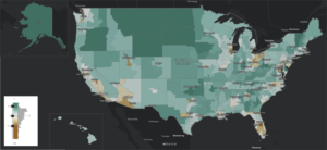
Using a statistical technique called factor analysis, we were able to create an index that incorporates all these measures and to determine the optimal weights for capturing as much information possible based on the correlations between variables. We call this the Natural Communities index. Not surprisingly, the results of the factor analysis suggested giving the most weight to sharing a boundary with an existing administrative boundary. The least weight was given to proximity to a mountain peak. Geographical compactness helps the score, but not by much since that measure was given such a low weight. The infrastructure measures both had sizeable negative weights, meaning that having infrastructure as a boundary is somehow negatively associated with our construct of natural communities and thus hurts a district’s score, perhaps because infrastructure is used to bring people together rather than separate them. Using these weights, we can come up with a “natural communities” score for each district. The scores were then standardized to have a mean of zero and a standard deviation of 1, for easy comparison. Districts that score high on our Natural Communities index are shown in green on the map below, whereas districts that score low are shown in brown.

States with only one district (Alaska, Delaware, Montana, North Dakota, South Dakota, Vermont, and Wyoming) generally scored highly, but these districts having different values does not make sense since there were no other options these districts could have used. We gave all these districts a “perfect” score of 2.0, shown in dark green in the map.

A Look at Specific Districts

New Mexico’s 1st

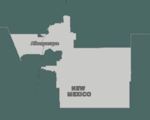
New Mexico’s 1^st District scored average (0). This district has 60.4 percent of its perimeter defined by administrative boundaries (national average was 65.4 percent), and 2.4 percent defined by a major highway (national average was 2.3 percent).

Ohio’s 3rd

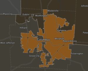
Ohio’s 3^rd District scored very low (-3.5). This district has only 16.3 percent of its perimeter defined by administrative boundaries (national average was 65.4 percent), and high percentages defined by the two infrastructure categories – railroad tracks and major highways – which has a negative impact on the score.

Arkansas’ 2nd

Arkansas’ 2^nd District scored very high (+1.4). This district has 100 percent of its perimeter defined by administrative boundaries (national average was 65.4 percent), zero percent defined by infrastructure, and 37.5 percent defined by a river or stream (national average was 18.1%).

Our index adds information by accounting for the existing administrative boundaries as well as considering infrastructure and physical geographic features. This new score provides much more context when evaluating congressional district boundaries than simply geographical compactness. For example, Arkansas’ 2^nd District is slightly less compact than New Mexico’s 1^st District but scores much higher when taking into account the existing administrative boundaries (counties and places) and physical geographic boundaries (rivers and mountain peaks).

Join the Discussion

Our natural communities score can be used going into the upcoming redistricting exercises when evaluating multiple proposed districts. This score can add to the conversation when communicating proposed plans to the public during briefings and comment periods.

For maps, data, and other resources for creating your own policy maps, visit Esri Maps for Public Policy or watch the video Top 10 Tips for Policy Story Maps.

About the Author

Diana C. Lavery is a product engineer on Esri’s Living Atlas and Policy Maps teams.